The Game of Life

Hello World!

Finally! I have been trying to start a dev blog for like 10 years now, and I always found a way to procrastinate that 😩.

I always thought I would never have the time or enough content to publish. But I've always been an enthusiast of generative art and algorithmic art, and one day it hit me: "Hey, that never goes old!". So here we are.

Usually the first thing you do when you start something technology-related is a Hello World of some sort. But this time around, I would like to do something related to generative art, as this blog is going to track all the progress and projects I do regarding that adventure. For that purpose, what better place to start than with Conway's The Game of Life! It is sort of the Hello World of generative art after all. (isn't it? 😅)

What is it?

For those of us who thought The Game of Life was an old family board game created by Milton Bradley, we need a little bit more of an introduction to Conway's version. Directly from its Wikipedia article:

The Game of Life is a cellular automaton devised by the British mathematician John Horton Conway in 1970. It is a zero-player game, meaning its evolution is determined entirely by its initial state. You interact with it by creating an initial configuration and observing how it evolves. It is Turing complete and can simulate a universal constructor or any other Turing machine.

That last part is really interesting — Turing complete. That means this tiny set of rules, applied to a grid of cells, can in theory compute anything a regular computer can. From nothing but a grid and four rules. And it produces incredible looking results that you can tweak endlessly through code ✨

The universe of the Game of Life is an infinite, two-dimensional grid of square cells. Each cell can either be alive or dead. Every cell interacts with its eight neighbors (horizontally, vertically, and diagonally adjacent). At each step in time, we evaluate the following rules:

1. Under-population: A live cell with fewer than two live neighbors dies.
2. Survival: A live cell with two or three live neighbors lives on.
3. Over-population: A live cell with more than three live neighbors dies.
4. Reproduction: A dead cell with exactly three live neighbors becomes alive.

Seems simple enough! But the magic lies in how these simple rules create massive, infinite complexity. We determine the initial state either manually or randomly, and then we just... watch it evolve. No player input. No decisions. Just pure emergent behavior from four lines of logic.

So... how do we actually code this? Let's do this!

The World is Flat

Once we start talking about 2D grids, our minds immediately jump to 2D arrays (e.g., state[x][y]). But here is the gotcha: there is no such thing as a 2D array for a computer. They are just mathematical constructs on top of arbitrary length data! Usually, the most resource-intensive part of graphics sketches is rendering, and traversing nested arrays pixel-by-pixel is slow.

Instead, let's use 1D arrays. This is how frame buffers and images are actually represented natively in computer graphics — one long flat buffer of pixels, row after row. Converting between 1D and 2D coordinates is straightforward:

// From 2D(x, y) to 1D(i)
i = y * width + x

// From 1D(i) to 2D(x, y)
x = i % width
y = floor(i / width)

We store each row of pixels one after the other, so we need the width to know where each row ends. One thing to note: that y could be a floating point number when dividing, and we can only index arrays with integers, so don't forget floor()! (I learned that one the hard way 😅)

And here is the coolest part: 1D arrays are already toroidally bound on the X-axis! 😲 What does that mean? It means if x == width and we do x + 1, instead of throwing an Out of Bounds error like a 2D array would, it seamlessly wraps to the first item of the next row. Just like Pac-Man going out one side of the screen and coming out the other! Not perfect (you end up a row below), but good enough for our grid — and way simpler than explicit boundary checking.

The Setup

We are going to use p5.js for this. From their site:

p5.js is a JavaScript library for creative coding, with a focus on making coding accessible and inclusive for artists, designers, educators, beginners, and anyone else!

Every sketch starts with two functions: setup and draw. Beyond that, everything else is just plain old JavaScript. Let's start by declaring our state arrays and the neighbor offsets.

Instead of using booleans right away, let's store the actual color values of our cells — 255 (white) for live, 0 (black) for dead. This has a sneaky benefit: 0 evaluates to false in JavaScript, so our conditionals still work, but we can also use the value directly for rendering.

let size;               // width * height (DRY)
let state, next;        // current and next generation
let percentage = 25;    // ~% of live cells to seed
let live = 255;         // color for live cells ('limegreen', '#FF6600')
let dead = 0;           // color for dead cells ('pink', 'rgba(123,45,67)')
let offset;             // hold the adjacent offsets of neighbours

function setup() {
    createCanvas(180, 120);
    frameRate(10);
    size = width * height;
    state = Array(size).fill(dead);
    next = Array(size).fill(dead);
    offset = [ // offsets for neighbours in 1D array
        -width - 1, // nw
        -width,     // n
        -width + 1, // ne
        1,          // e
        width + 1,  // se
        width,      // s
        width - 1,  // sw
        -1,         // w
    ];
    seed();
}

Let's talk about that offset array — it's one of my favorite tricks in this whole implementation. Accessing neighbors in a 2D array means checking 8 different [x+dx][y+dy] combinations. But in a 1D array, each neighbor is just a simple arithmetic offset from the current index:

state[i - 1]            // west
state[i + 1]            // east
state[i - width]        // north (one full row back)
state[i + width]        // south (one full row forward)
state[i - width - 1]    // northwest
state[i - width + 1]    // northeast
state[i + width - 1]    // southwest
state[i + width + 1]    // southeast

Since only i changes and the offsets are constants (once width is known), we precompute them into that array and just iterate over it. No nested loops, no boundary math, just i + offset[j].

Initialization

In a 2D array, randomly seeding live cells means looping over X and Y and rolling a dice for each cell (like flipping a coin). This usually nets you exactly ~50% alive/dead population.

But with 1D arrays? We can just calculate the literal number of cells we want alive based on a percentage, pick N random index spots, and turn them on! Faster, simpler, and way more flexible.

(A quick gotcha: p5.js's random() function returns floating point numbers! So remember to floor it before you try indexing your array, or JavaScript will be very unhappy).

// Randomly seeds the state with live cells
function seed() {
    state.fill(dead);
    const living = floor(size * percentage / 100);
    for (let i = 0; i < living; i++) {
        state[floor(random(size))] = live;
    }
}

The Rules of Life

Every step we must iterate over each cell, count its live neighbors, and apply Conway's rules. Using our offset array, this becomes beautifully simple.

But first, we need a little helper. Remember how the 1D array only natively wraps on the X-axis? For the Y-axis, we need to handle it manually. Enter the at(i) function:

// Gets cell 'status' at a given index (1D)
function at(i) {
    if (i < 0) i += size;
    if (i >= size) i -= size;
    return state[i] == live ? 1 : 0;
}

What's happening here? If the index goes negative (above the top row), we add size to wrap it to the bottom. If it exceeds size (below the bottom row), we subtract size to wrap it to the top. Then we return 1 for alive, 0 for dead — perfect for summing up neighbors.

Then during each step, we apply the rules to generate the next state. The formatting looks a little weird, but I did it on purpose for readability — each of Conway's four rules maps to exactly one line:

// Creates the next generation of cells
function step() {
    for (let i = 0; i < size; i++) {
        let neighbours = 0;
        for (let j of offset) {
            neighbours += at(i + j);
        }
        if ((state[i] == live) && (neighbours < 2)) next[i] = dead;     // under-population
        else if ((state[i] == live) && (neighbours > 3)) next[i] = dead;     // over-population
        else if ((state[i] == dead) && (neighbours == 3)) next[i] = live;     // reproduction
        else next[i] = state[i]; // stasis
    }
    let tmp = state;
    state = next;
    next = tmp;
}

Notice the swap at the end: instead of creating a new array every frame (expensive!), we maintain two arrays and just swap references. The "next" generation becomes the "current," and the old "current" gets recycled as scratch space.

Drawing

Because our logic is blazing fast, the rendering is a single-loop assignment. We convert each 1D index back to 2D coordinates inline and set the pixel color directly from the state value:

// Main rendering loop
function draw() {
    for (let i = 0; i < size; i++) {
        set(i % width, floor(i / width), color(state[i]));
    }
    updatePixels();
    step();
}

The set(x, y, color) function writes directly to the pixel buffer, and updatePixels() flushes the whole frame at once. Because we stored the color value (255/0) directly in the state array, we don't need any conditionals — just color(state[i]).

Now check it out!

Simple Life View on GitHub

Click anywhere on the canvas to re-seed it!

The initial state is randomly seeded with 25% live cells, and then we let the game follow its course. I used frameRate(10) so that each generation could be appreciated.

If you try this code in the p5.js web editor, you'll notice the sketch is really small — exactly 180×120 pixels as defined in setup. Your first instinct would be to bump up createCanvas(1280, 720), but that doesn't scale the pixels — it just gives you way more cells (and way more computation). The trick is that the browser can scale the <canvas> element independently of its resolution! I'm using CSS to stretch it to full width:

canvas {
    width: 100% !important;
    height: 100% !important;
    image-rendering: pixelated;
}

That image-rendering: pixelated is the secret sauce — it disables interpolation so our tiny pixels don't blur into each other when scaled up. They stay as perfect, crisp squares. (Some browsers call this crisp-edges, but pixelated works in all modern ones now 🎉)

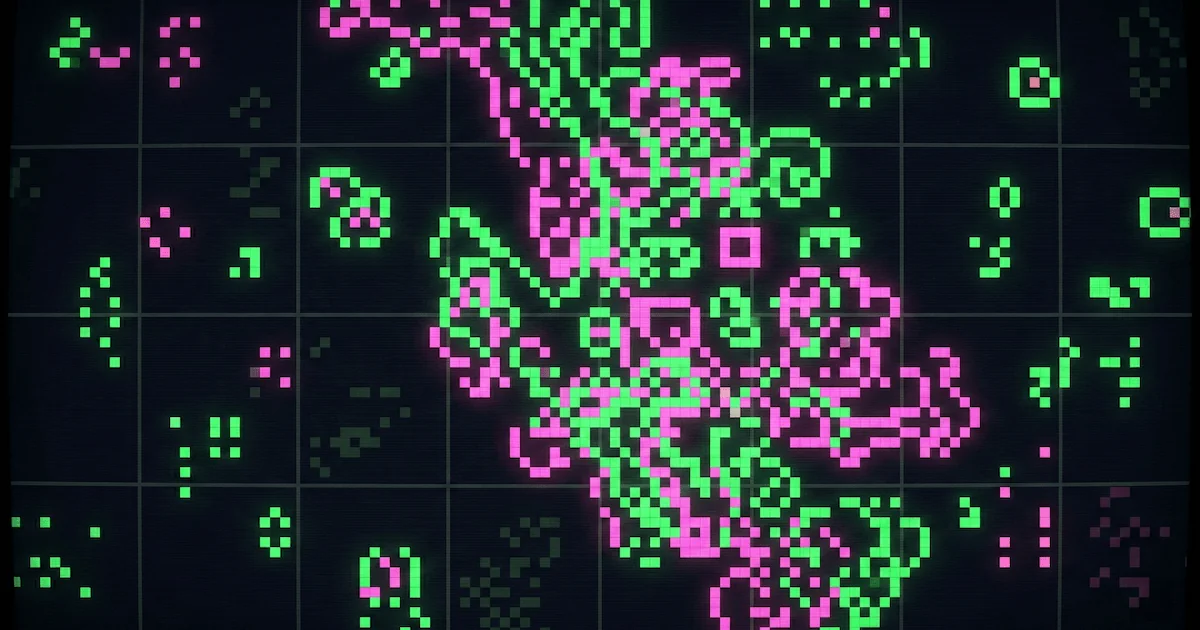
Making it Colorful (and Interactive!)

Okay, there is not much "art" in diminutive black and white pixels dancing around a tiny canvas (or... is there? 🤔). Thankfully, because we implemented this grid so cleanly, manipulating the visuals is a breeze.

First, some structural changes. We grow the canvas to a comfortable 1280×720, and introduce a resolution variable that creates a "virtual grid" on top of the canvas. With resolution = 10, our actual cell grid becomes 128×72 — a nice size to play with. And since we're drawing shapes now instead of raw pixels, we switch live/dead from integers to booleans. (The rest of the code works without a hitch because false is falsy in JavaScript — same behavior, cleaner semantics.)

The real magic happens in the rendering. Instead of setting individual pixels, we only draw the live cells as colored circles. We skip dead cells completely (way more efficient than clearing and drawing everything). And for the color? We map the cell's 1D index to the HSL hue spectrum — map(i, 0, size, 0, 360). That's it. Instant rainbow 🌈

// Main rendering loop
function draw() {
    if (mouseIsPressed === true && mouseX >= 0 && mouseX <= width && mouseY >= 0 && mouseY <= height) {
        let i = floor(mouseY / resolution) * w + floor(mouseX / resolution);
        if (i >= 0 && i < size) {
            state[i] = live;
            cell(i, mouseX, mouseY);
            return;
        }
    }

    clear();
    background(0);
    for (let i = 0; i < size; i++) {
        if (state[i]) {
            let x = (i % w) * resolution;
            let y = floor(i / w) * resolution;
            cell(i, x, y);
        }
    }
    step();
}

// Draws a colored circle with interpolated hue
function cell(i, x, y) {
    fill(`hsl(${floor(map(i, 0, size, 0, 360))},100%,50%)`);
    circle(floor(x) + half, floor(y) + half, resolution);
}

The cell(i, x, y) function interpolates i into a hue value [0°, 360°), creating a smooth gradient across the entire grid. And notice the mouseIsPressed check at the top of draw — when you click and drag, it converts mouse coordinates back to grid coordinates and seeds live cells directly into the current generation. You can literally paint life onto the canvas while it evolves.

The result? A clear winner 🏆

Colorful Life View on GitHub

Click and drag your mouse across the canvas to magically paint new life!

Now we're talking! Try clicking and dragging your mouse across the paused cells above to "paint" new life structures dynamically and watch them explode.

Closing Thoughts

Experimenting with simple rules that result in infinite complexity is incredibly satisfying. Four rules. That's it. No physics engine, no AI, no complex state machines. Just four conditionals applied to a grid, and the system produces gliders, oscillators, spaceships, and patterns that mathematicians are still discovering 55 years later.

I really enjoyed writing Life and I will definitely keep doing these visual algorithms! There are hundreds of implementations all over the internet — even one in the Go documentation and another in the p5.js examples. But there's something deeply satisfying about writing your own from scratch, making design decisions like 1D arrays over 2D, and discovering tricks like the offset array along the way.

In a future post, I might push this into WebAssembly with Go to see how many millions of cells we can crank at 60FPS. Or maybe explore other cellular automata like Langton's Ant or Rule 110 — another Turing complete system, but this time in just one dimension. (How wild is that? 😲)

¡Hasta la próxima!